Background
Throughout this post, we follow the standard mathematical convention that vectors are represented as column vectors, not row vectors. We’ll start by understanding self-attention for a single token, then generalize to the batched matrix form used in practice.
Single Token Self-Attention
Consider a sentence with $N$ tokens: $[t_1, t_2, \cdots, t_i, \cdots, t_N]$. For a single token $t_i$, its embedding is $\mathbf{x}_i \in \mathbb{R}^d$. The question is: how do we compute its output vector $\mathbf{z}_i \in \mathbb{R}^{d_2}$ after applying self-attention?
Deriving Query, Key, and Value Vectors
Starting from the token $t_i$, we first represent it as a one-hot vector of length $|V|$ (where $|V|$ is the vocabulary size). We then obtain its embedding using a learnable embedding matrix $W_E \in \mathbb{R}^{d \times |V|}$:
$$\mathbf{x}_i = W_E t_i \tag{1}$$Important: Although this looks like matrix multiplication, it’s actually just an index lookup operation, not a full matrix multiplication. Since $t_i$ is one-hot, $W_E t_i$ simply selects the corresponding column from $W_E$. This is extremely fast in practice—it’s a table lookup, not arithmetic.
In PyTorch, this is implemented using the torch.nn.Embedding layer:
embedding = torch.nn.Embedding(num_embeddings=|V|, embedding_dim=d)
x_i = embedding(token_id) # O(1) lookup, very fastFrom the embedding $\mathbf{x}_i$, we derive three learnable vectors using three separate linear transformations with learnable weight matrices:
$$\mathbf{q}_i = W_Q \mathbf{x}_i, \quad \mathbf{k}_i = W_K \mathbf{x}_i, \quad \mathbf{v}_i = W_V \mathbf{x}_i \tag{2}$$where:
- $W_Q \in \mathbb{R}^{d_1 \times d}$ projects embeddings to the query space
- $W_K \in \mathbb{R}^{d_1 \times d}$ projects embeddings to the key space
- $W_V \in \mathbb{R}^{d_2 \times d}$ projects embeddings to the value space
These projection matrices are learned during training and are the same across all tokens in a sequence.
The output $\mathbf{z}_i$ is a weighted sum of all value vectors. The weights should reflect how much each token contributes to the current token’s representation:
$$ \mathbf{z}_i = \sum_{j=1}^{N} w_j^i\mathbf{v}_j \tag{3} $$A natural choice for the weights $w_j^i$ is the dot product between the current token’s query and each token’s key The terminology is suggestive: a query searches over all keys by computing dot products. Matching keys produce high values. : $w_j^i = \mathbf{q}_i^T\mathbf{k}_j$.
This gives us the single-token attention equation:
$$ \mathbf{z}_i^T = \sum_{j=1}^{N} (\mathbf{q}_i^T\mathbf{k}_j)\mathbf{v}_j^T \tag{4} $$Batched Matrix Form
In practice, we process multiple tokens simultaneously using matrix operations. This is essential for GPU efficiency, as matrix multiplications are highly optimized compared to scalar operations.
Let’s denote the stacked embedding matrix as:
$$\mathbf{X} = \begin{bmatrix} \mathbf{x}_1^T \\ \vdots \\ \mathbf{x}_N^T \end{bmatrix}_{N \times d} \tag{5}$$The query, key, and value matrices are then obtained via linear transformations:
$$\mathbf{Q} = \mathbf{X} W_Q^T, \quad \mathbf{K} = \mathbf{X} W_K^T, \quad \mathbf{V} = \mathbf{X} W_V^T \tag{6}$$where $W_Q, W_K, W_V$ are the learnable weight matrices of shapes $d_1 \times d$, $d_1 \times d$, and $d_2 \times d$ respectively.
We can also stack all token vectors into a matrix using the standard convention:
$$\mathbf{D} = \begin{bmatrix} \mathbf{d}_1^T \\ \vdots \\ \mathbf{d}_N^T \end{bmatrix} \tag{7}$$The matrix forms are:
$$ \mathbf{Q} = \begin{bmatrix} \mathbf{q}_1^T \\ \vdots \\ \mathbf{q}_N^T \end{bmatrix}_{N \times d_1}, \quad \mathbf{K} = \begin{bmatrix} \mathbf{k}_1^T \\ \vdots \\ \mathbf{k}_N^T \end{bmatrix}_{N \times d_1}, \quad \mathbf{V} = \begin{bmatrix} \mathbf{v}_1^T \\ \vdots \\ \mathbf{v}_N^T \end{bmatrix}_{N \times d_2} \tag{8} $$Key insight: From this point forward, treat $\mathbf{q}_i$, $\mathbf{k}_i$, and $\mathbf{v}_i$ as atomic units. We don’t decompose them into individual scalar elements.
Computing Attention Weights
First, we compute pairwise similarities between all queries and keys. The matrix with $(i,j)$-th element equal to $\mathbf{q}_i^T\mathbf{k}_j$ is simply the matrix product:
$$\mathbf{QK}^T \tag{9}$$This is visualized in Figure 1: for each position $(i,j)$, we compute the dot product by looking left (to $\mathbf{Q}$’s $i$-th row) and up (to $\mathbf{K}^T$’s $j$-th column).
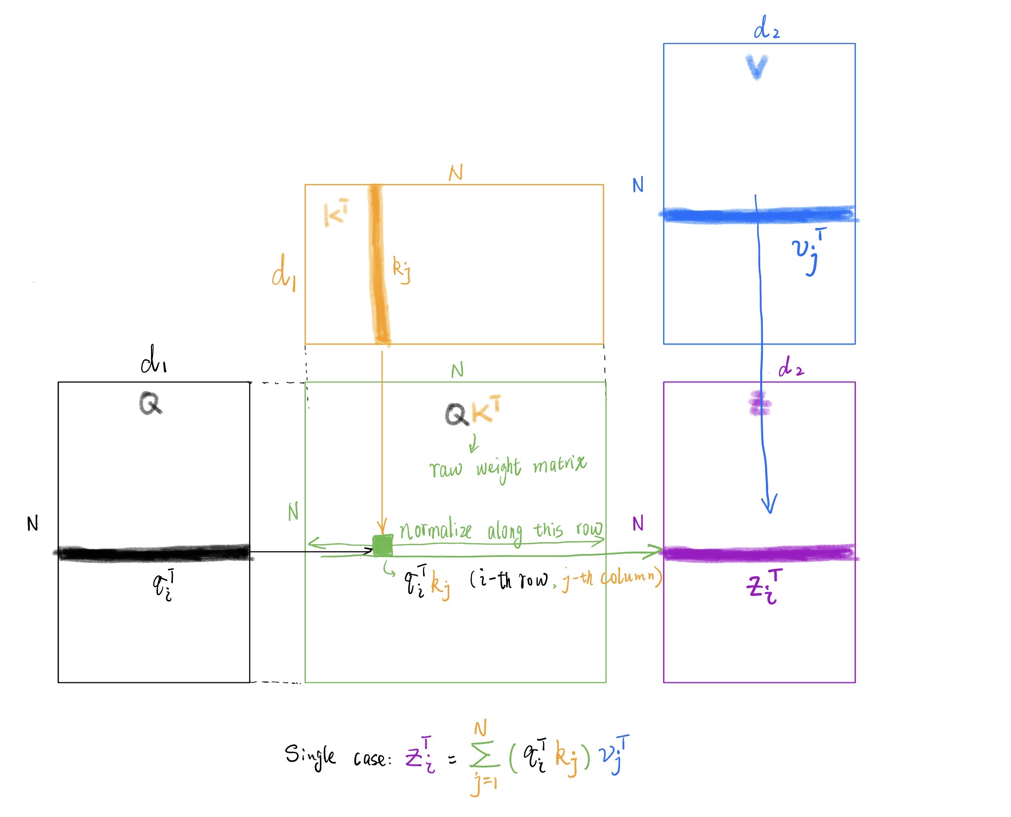
Figure 1: Self attention computation flow
Computing the Output
Next, we weight the value vectors by the attention weights. Note that in our single-token equation, we used transposes: $\mathbf{q}_i^T$ and $\mathbf{v}_j^T$. Following the matrix stacking convention, both $\mathbf{Q}$ and $\mathbf{V}$ are stored without transpose.
The output matrix is:
$$ \mathbf{Z} = \begin{bmatrix} \mathbf{z}_1^T \\ \vdots \\ \mathbf{z}_N^T \end{bmatrix}_{N \times d_2} \tag{10} $$For each row $\mathbf{z}_i^T$:
- Left: the attention weights for token $i$: $[\mathbf{q}_i^T\mathbf{k}_1, \cdots, \mathbf{q}_i^T\mathbf{k}_N]$ (the $i$-th row of $\mathbf{QK}^T$)
- Up: the value vectors: $[\mathbf{v}_1^T, \cdots, \mathbf{v}_N^T]$ (the rows of $\mathbf{V}$)
Multiplying these gives exactly the single-token case we derived earlier.
Final Form
Reading the matrix multiplication from left to right:
$$ \mathbf{Z} = (\mathbf{Q}\mathbf{K}^T)\mathbf{V} \tag{11} $$Or, substituting the definitions of $\mathbf{Q}$, $\mathbf{K}$, $\mathbf{V}$ in terms of the embedding matrix $\mathbf{X}$ and weight matrices:
$$ \mathbf{Z} = ((\mathbf{X} W_Q^T)(\mathbf{X} W_K^T)^T)(\mathbf{X} W_V^T) = ((\mathbf{X} W_Q^T)(W_K \mathbf{X}^T))(\mathbf{X} W_V^T) \tag{12} $$This end-to-end equation shows how the output embeddings $\mathbf{Z}$ are derived from the input embeddings $\mathbf{X}$ through three learnable weight matrices $W_Q$, $W_K$, and $W_V$.
Note: This derivation omits softmax normalization, scaling (by $\sqrt{d_1}$), and masking—important details for real implementations, but easy to incorporate once this foundation is clear.